Pipeline Predictive Maintenance: Sensor Strategies, Failure Modes, and AI Models

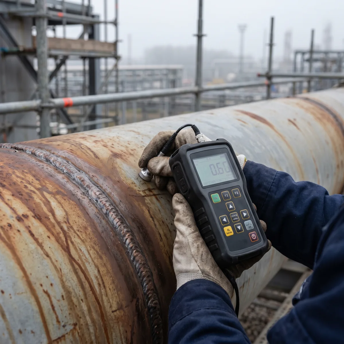
Pipelines fail through a small, well-characterized set of mechanisms — internal and external corrosion, third-party mechanical damage, stress corrosion cracking, weld and material defects — and each one leaves a different signature in the data, on a different timescale, best caught by a different sensing strategy. Treating "pipeline predictive maintenance" as a single monitoring problem is why so many programmes end up with a system that is excellent at catching sudden pressure transients and nearly blind to a corrosion pit that has been thinning a wall section for three years.

"IoT sensors plus AI" undersells how failure-mode-specific pipeline monitoring actually is — a leak-detection system and a corrosion-forecasting system solve different problems, on different signals, at different timescales.

§ 02SCADA and Pressure-Signal Anomaly Detection

Leak detection is the fast-timescale problem: negative pressure wave analysis and real-time mass-balance methods can flag a rupture within seconds to minutes by watching for the pressure transient a sudden loss of containment produces, or for a sustained mismatch between metered inflow and outflow. The practical engineering question is rarely whether to add sensors — most operators already have SCADA pressure and flow instrumentation — but how to tune detection sensitivity against the pipeline's own operational noise: pump starts, valve operations, and demand swings all produce pressure signatures that a naively-tuned detector confuses with a leak, which is what pushes most false-alarm rates in early deployments.

§ 03Corrosion-Rate Forecasting from Inline Inspection Data

Corrosion is the slow-timescale problem, and the primary data source is different in kind: inline inspection ("smart pig") runs that measure wall-thickness loss at thousands of points along a pipeline segment, repeated every few years. The forecasting task is to fit a corrosion-growth model — typically a rate per unit time, sometimes accelerating where coating damage or microbial activity compounds the loss — to successive ILI runs, and project each defect's remaining wall thickness forward against the pipeline's design pressure rating. The accuracy ceiling here is set less by modelling sophistication than by ILI run frequency: a growth-rate estimate from two inspection runs eight years apart is far less reliable than one from three runs at closer intervals, which is the trade-off operators are actually making when they set inspection cadence.

§ 04From Anomaly Flags to Burst-Risk Scoring

The step that turns either data stream into a maintenance decision is combining a defect's forecasted severity with the pipeline's operating conditions — pressure, diameter, wall thickness, material grade — into a burst-risk score using established structural models such as B31G or its modified variants, then ranking defects across the network by that score rather than by raw wall-loss percentage alone. Two defects with identical wall-loss readings can carry very different burst risk depending on the pressure they operate under, and a ranked, risk-weighted worklist is what actually lets a limited repair budget go to the segments where a failure would matter most, rather than to whichever defect happened to be found first.